Noisy Grids

Thinking about flow in Processing (more on that to follow) perlin noise visualisation continues to be fascinating. Here are some examples in an x-y grid setting using a basic set of points shown as circles in an arrangement across and down the screen.

No Noise

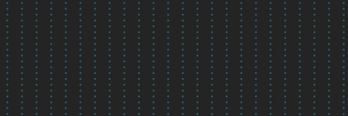
First we have the normal grid pattern with some pleasing colour choices:

size(1190, 397)

background_colour = color(36, 36, 36) 
background(background_colour)
fill(background_colour)

stroke_colour = color(51, 160, 195)
stroke(stroke_colour)

radius = 5
xspacing = 50
yspacing = 20
noise_increment = 0.01
xoff = 0.0
yoff = 0.0

lastx = -1
lasty = -1

for y in range(yspacing/2, height, yspacing):
    lasty = -1
    lasty = -1
    xoff = 0.0
    
    for x in range (xspacing/2, width, xspacing):
        xvalue = x
        yvalue = y
        
        circle(xvalue, yvalue, radius)
        
        xoff += noise_increment
        lastx = xvalue
        lasty = yvalue
        
    yoff += noise_increment

Note some unused variables lastx, lasty, xoff, yoff, noise_increment are there to make the code work when we introduce some pertubation later.

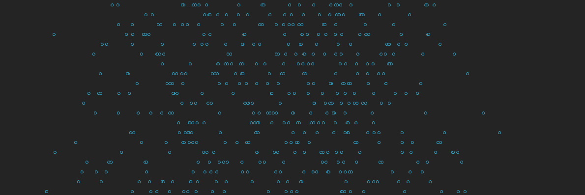
X Perlin Noise

Adding perlin noise, we map values we get from the noise function from 0..1 to the width and height of the screen. If we apply noise to the x values:

    for x in range (xspacing/2, width, xspacing):
        xvalue = map(noise(x, y, xoff), 0, 1, 0, width)
        yvalue = y
            

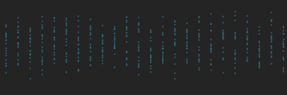
Y Perlin Noise

Similarly if we keep x fixed and add noise to the y values:

    for x in range (xspacing/2, width, xspacing):
        xvalue = x
        yvalue = map(noise(x, y, yoff), 0, 1, 0, height)

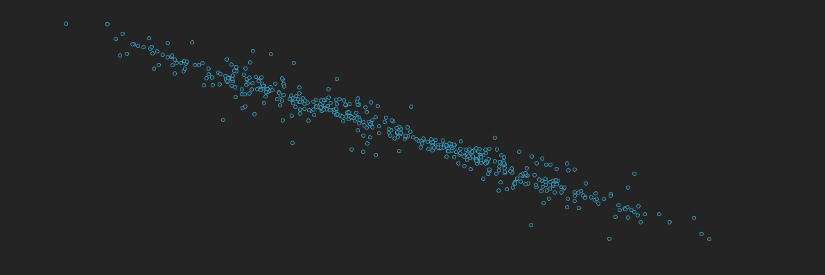
X & Y Perlin Noise

And as you might imagine if we add noise to both, the most interesting pattern emerges, something like a photo of the tilt of the milky way.

    for x in range (xspacing/2, width, xspacing):
        xvalue = map(noise(x, y, xoff), 0, 1, 0, width)
        yvalue = map(noise(x, y, yoff), 0, 1, 0, height)